How to price tokens with Buybacks & Burns

A framework to help you price tokens with buybacks and burns, along with a case study of Hyperliquid which sets HYPE price anchor at $105

Introduction

Crypto tokens have often been perceived as difficult to value. Many tokens on the market are considered meme tokens with limited utility within their respective protocols. Frequently, these tokens serve primarily as a mechanism for protocol developers to exit early, which has contributed to shorter lifespans for many crypto projects. In numerous instances, projects that launch with high token valuations become inactive when founders leave prematurely, leaving insufficient incentives for continued development. These challenges largely arise from the highly speculative nature of the crypto market, where the direct transfer of value from the protocol to the token is frequently uncertain.

A recommended strategy for ensuring value flows from protocol to token involves implementing token buybacks and burns. While commonly referred to as “scarcity mechanics,” token buybacks and burns can be rigorously analyzed as a discounted stream of value capture, drawing a parallel to equity buybacks. However, it is important to note that tokenholders typically do not possess a legal claim on cash flows, meaning this model serves more as a fundamental anchor (“fee-backed value”) than as a guaranteed pricing mechanism.

This article introduces a clear, two-stage methodology for valuing a token when a portion of protocol fees are allocated to buy back—and potentially burn—the token, alongside scenarios where fee growth is fueled by reinvestment over a finite period before transitioning to a stable growth phase.

We conclude by examining Hyperliquid as a case study and providing an estimated token price of $105 based on current burn rates.

Additionally, we will explore the impact of varying burn rates on price and offer recommendations for an optimal burn rate for Hyperliquid. This approach is not applicable for tokens such as Bitcoin, Ethereum where they are native fee tokens of the chain and their value is driven by the activity on the chain. The transfer of value in such cases happen when user pays fees in the native token for an activity on the chain.

The Core Idea: Present value of buybacks

Buybacks and burns allow a protocol to permanently convert its revenue into value for its token. This process is considered permanent because, once the tokens are bought back and destroyed, their value cannot be recovered from the market. Burns play a key role in transferring value. The approach depends largely on analysing the protocol’s income—specifically, the fees it generates—and then determining what proportion of those fees is used for buybacks and burns. Using part of the fees for buybacks leads to some surprising metrics in token valuation, which may not appeal to most market participants.

Let us assume the protocol generates annual fees F_t (in USD terms) at time t. A fraction p of fees is allocated to buybacks BB_t:

$$BB_t = p \cdot F_t$$

If you treat these buyback dollars as the economic “payout equivalent” to tokenholders, then the intrinsic anchor for the token’s value is the present value of buybacks:

$$PV_{BB} = \sum_{t=1}^{\infty} \frac{BB_t}{(1+r)^t}$$

where r is the discount rate capturing time value and risk (for crypto, this is typically much higher than risk-free rates). Finally, to translate from total PV into per-token value, divide by supply S (choose either circulating or total, but be consistent):

$$P^* = \frac{PV_{BB}}{S}$$

This is the conceptual foundation: the token is “worth” the discounted value of expected future fee-funded buybacks, spread across the token base.

Modeling Fees: A Two-Stage Growth Process

The key driver is the fee path F_t. Our two-stage structure is:

1. Early stage (years 1 to T): the protocol is still scaling, and reinvestment is productive.
2. Mature stage (years T+1 onward): reinvestment-driven growth shuts off (or becomes negligible), and fees grow at a stable mature rate.

Inputs

• F₀: fees “today” (your starting annual fees)
• p: buyback rate (fraction of fees used to buy back)
• 𝜌: ROIC in the early stage (return on reinvested capital)
• g_E: early-stage baseline fee growth (organic adoption, market growth, etc.)
• g_L: mature-stage baseline fee growth (terminal growth)
• r: discount rate
• T: number of early-stage years

How reinvestment maps into growth

If the protocol buys back fraction p, it retains fraction (1 − p) to fund growth. In the early stage, retained capital produces incremental fee growth at rate:

$$\text{incremental growth} = (1-p)\rho$$

This is a standard formula used to derive growth based on reinvestment in corporate finance. So the total early-stage fee growth factor is:

$$A = 1 + g_E + (1-p)\rho$$

In the mature stage, incremental ROIC is assumed to be 0 (or treated as already competed away), so fees grow at:

$$B = 1 + g_L$$

Discount factor is defined as:

$$D = 1 + r$$

With these definitions, fees evolve as:

$$F_t =\begin{cases}F_0 A^{t}, & t = 1,2,\ldots,T,\\[4pt]F_0 A^{T} B^{,t-T}, & t= T+1, T+2, \ldots, \infty.\end{cases}$$

where the first stage can be defined as early high growth stage and second stage can be defined as mature stage.

Discounting the Buybacks

Since buybacks are a constant fraction p of fees, buybacks in year t are:

$$BB_t = pF_t$$

The present value of these buybacks can be defined as:

$$PV_{BB} = \sum_{t=1}^{\infty} \frac{pF_t}{D^t}$$

We split this into:

• PV₁: years (1..T)
• PV₂: years (T+1.. ∞)

High Growth Stage Present Value: Years 1..T

Substitute F_t = F₀A^t:

This is a geometric series. For A ≠ D:

Mature Stage Present Value: Years (T+1.. ∞)

For t >T, F_t = F₀A^TB^t-T. then:

Let k= t-T so k=1,2,...:

The infinite geometric sum converges only if:

If g_L < r, then:

So:

The Fair Pricing Formula

The “fair price” per token is PV of buybacks divided by supply S:

$$P^* = \frac{PV_1 + PV_2}{S}$$

Substitute PV₁ and PV₂:

with:

• A = 1 + g_E + (1-p) 𝜌, capped at some sensible A_max
• B = 1 + g_L
• D = 1 + r

and the required convergence condition g_L < r. A should be capped at some sensible value because otherwise the fees generated could end up growing to some insensible values.

Interpreting the Components

The first term: “high-growth years”

$$\frac{\frac{A}{D}\left(1-\left(\frac{A}{D}\right)^{T}\right)}{1-\frac{A}{D}}$$

captures the discounted value of buybacks during the period when reinvestment has high marginal impact.

The second term: “terminal value”

$$\left(\frac{A}{D}\right)^{T} \frac{B}{D-B}$$

is a textbook terminal value, but expressed in a way that is consistent with buyback cash flows rather than dividends. It is the mature “forever” component, discounted back through the early-growth period.

One of the intresting observations which can derived from this model, is that if there are no buyback and burns then p = 0, which implies the price of the token should be 0. In this model we have entirely discounted the value which can be ascribed to governance etc. The reason is simple, governance doesn’t imply value transfer to the token holders. If you hold shares of a company which gives you voting right but no right to profits etc, then whats the point of those voting rights? The only reason those voting rights can be useful is if the token holders can use those rights to benefit themselves.

Practical Modeling Guidance

Choose the supply basis deliberately

• If you divide by circulating supply, your P^* is closer to a market-comparable “per circulating token” anchor.
• If you divide by total/FDV supply, you get a more conservative FDV-style anchor.

Discount rate matters more in crypto

Because token holder rights are not contractual in the same way as equity, the discount rate r should incorporate:

• protocol risk (competition, tech, security),
• policy risk (will buybacks persist?),
• regulatory risk,
• market regime risk.

Validate fee inputs

Fee series are volatile and can be noisy. The model is only as good as F₀, g_E, g_L, and the realism of assuming that buybacks remain a stable fraction p of fees.

Ensure g_L < r

If terminal growth exceeds the discount rate, the terminal value becomes mathematically unstable and economically implausible.

What This Model Does—and Does Not—Claim

What it does - Provides a fundamental value anchor for a buyback token: “If buybacks track fees and fees grow as modeled, this is the PV of buybacks per token.”

What it does not - Guarantee market price. Crypto markets can and do trade at premiums or discounts to fee-backed value due to optionality, narrative, collateral demand, reflexivity, and liquidity effects.

Hyperliquid

Lets study Hyperliquid token under this framework. I will avoid giving a lot of introduction about the protocol and straight away dive into laying out the model parameters and their justification. These parameters are based on the state of the protocol as of date of writing of this article 23 Dec, 2025

• Fees (F0): USD 1 Billion, Hyperliquid generated around USD 1 Billion in fees in year 2025
• Buyback Rate (p): 97%, this is the current rate at which Hyperliquid buybacks tokens
• ROIC(𝜌): 80%, quite standard for such high growth startups
• Early Base Growth Rate (gE): 30%, this is the growth rate Hyperliquid can achieve because of organic factors such as community etc.
• Mature Growth Rate: 5%
• Discount Rate (r): 20%, because of the high risk nature of the investment
• Amax: 150%, we assume that the growth rate of the protocol in early stage cannot be more than 50%
• T: 10 years, We value early stage as 10 years
• Supply(S): 336 Million, as described on CoinMarketCap

Under these assumptions, we get PV₁ = USD 17.33 Billion and PV₂ = USD 18.15 Billion, resulting in a total PV of USD 35.48 Billion and a token price of USD 105. We believe these are fair assumptions. You can modify them to suit your beliefs and come up with your own price target.

Effect of Buybacks

Beyond just the price target, the impact of buybacks is particularly worth examining. According to the previous assumptions, the highest token price occurs when around 75% of funds are allocated to buybacks. This outcome is influenced by the growth rate achieved as reinvestments in the project increase. If profits are not reinvested into the business, this leads to slower growth and, consequently, a lower token price. This issue has been a persistent concern within the Hyperliquid community, and it appears to be justified. The remaining 25% of cash could be used by the Hyperliquid team for marketing or even distributed as airdrops to existing traders on the platform, rewarding their contributions. In value terms, this 25% equates to roughly USD 250 million—a significant amount for an airdrop by any measure. Given trends in the cryptocurrency market, substantial trading activity often stems from anticipation of such airdrops. If Hyperliquid continues its airdrop program, competing platforms may find it challenging to attract attention, which could further accelerate Hyperliquid’s growth.

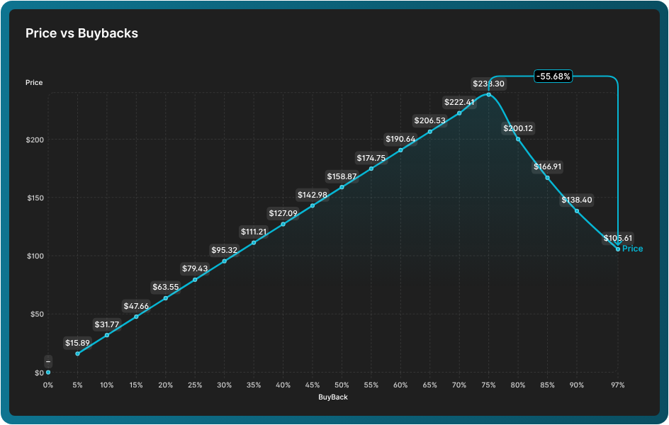
Also, in the absence of A_max the buyback percentage comes to around 20%, but at those rates we see that fees generated by the protocol becomes so large so soon that the model stops making sense. Capping A at 150% seems sensible and yes, the value 75% of buyback is also being driven by this cap.

Effects of Supply

Another key consideration is whether to base the token’s valuation on circulating supply or total supply. At present, there are about 336 million Hyperliquid tokens in circulation. With upcoming team unlocks, the supply would double, causing the price target to drop to approximately USD 55. There has been considerable discussion about these team unlocks, but according to this model, even with these releases, the token price should remain around USD 55.

Effects of Growth Rate - Bull & Bear Case

Lately, competition has been heating up for Hyperliquid. Considering, the number of perp dexes which are propping up everyday, Hyperliquid is poised to loose a considerable market share. That being said, so far the rate at which Hyperliquid has been innovating and delivering products is almost unparallel in perp-dex space. Exchanges tend to operate on networking effects and it’s not easy to build two sided liquidity. Once a threshold is achieved users will tend to stick around for better liquidity and execution.

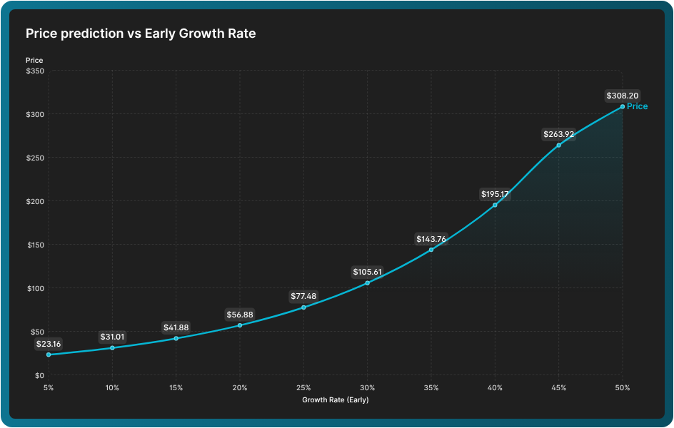
The above graph shows affect of growth rate will have on our predicted price. The bear scenario where Hyperliquid only grows at a base early growth rate of 5% puts the price prediction at USD 23 which is very close to the price it is trading at currently. But, if Hyperliquid is able to maintain its lead position and grows at a rate of say 50%, the predicted price would be USD 308.

Conclusion

This article has sought to establish a framework for token valuation, drawing significant inspiration from the discounted cash flow (DCF) model commonly used in equity valuation. Consequently, this approach inherits both the advantages and limitations of DCF. The model enables the optimization of an appropriate buyback rate, and also highlights the potential benefits of ongoing airdrops or allocating a portion of generated fees towards marketing initiatives. These measures can organically increase protocol fee generation and positively influence token pricing. Hyperliquid serves as a compelling case study for this framework, given its unprecedented scale and transparency in implementing buybacks within the crypto community. While Binance operates a substantial buyback and burn program, it does not match Hyperliquid’s level of transparency. In the months ahead, multiple perpetual decentralized exchanges are expected to launch. We hope these platforms will adopt lessons from Hyperliquid by incorporating consistent buyback and burn mechanisms.

Disclaimer

We are holders of the Hyperliquid token, and projecting optimistic price targets for the token may serve our interests. We are mostly doing mid frequency strategies on Hyperliquid with lower volumes and higher holding time frames. Our expectation of any airdrop going forward if enabled is pretty low. We strongly encourage readers to conduct their own research and reach independent conclusions.